There are two different ways to change the characteristics of a PWM waveform:
-
Synchronous Update: If no time base changes are required, you can use a synchronous update. With a synchronous update, the change in the waveform characteristics occurs on a cycle boundary, providing a smooth transition.
-
Asynchronous Update: Typically with PWM operation, the pulse width is varied while the cycle time remains constant so time base changes are not required. However, if a change in the time base of the PTO/PWM generator is required, an asynchronous update is used. An asynchronous update causes the PTO/PWM generator to be disabled momentarily, asynchronous to the PWM waveform. This can cause undesirable jitter in the controlled device. For that reason, synchronous PWM updates are recommended. Choose a time base that you expect to work for all of your anticipated cycle time values.
Tip The PWM Update Method bit (SM67.4 or SM77.4) in the control byte specifies the update type used when the PLS instruction is executed to invoke changes. If the time base is changed, an asynchronous update occurs regardless of the state of the PWM Update Method bit.
Using SM Locations to Configure and Control the PTO/PWM Operation
The PLS instruction reads the data stored in the specified SM memory locations and programs the PTO/PWM generator accordingly. SMB67 controls PTO 0 or PWM 0, and SMB77 controls PTO 1 or PWM 1. Table 6-36 describes the registers used to control the PTO/PWM operation. You can use Table 6-37 as a quick reference to determine the value to place in the PTO/PWM control register to invoke the desired operation.
You can change the characteristics of a PTO or PWM waveform by modifying the locations in the SM area (including the control byte) and then executing the PLS instruction. You can disable the generation of a PTO or PWM waveform at any time by writing 0 to the PTO/PWM enable bit of the control byte (SM67.7 or SM77.7) and then executing the PLS instruction.
The PTO Idle bit in the status byte (SM66.7 or SM76.7) is provided to indicate the completion of the programmed pulse train. In addition, an interrupt routine can be invoked upon the completion of a pulse train. (Refer to the descriptions of the Interrupt instructions and the Communications instructions.) If you are using the multiple segment operation, the interrupt routine is invoked upon completion of the profile table.
The following conditions set SM66.4 (or SM76.4) and SM66.5 (or SM76.5):
-
Specifying a cycle time delta value that results in an illegal cycle time after a number of pulses generates a mathematical overflow condition that terminates the PTO function and sets the Delta Calculation Error bit (SM66.4 or SM76.4) to 1. The output reverts to image register control.
-
Manually aborting (disabling) a PTO profile in progress sets the User Abort bit (SM66.5 or SM76.5) to 1.
-
Attempting to load the pipeline while it is full sets the PTO/PWM overflow bit (SM66.6 or SM76.6) to 1. You must clear this bit manually after an overflow is detected if you want to detect subsequent overflows. The transition to RUN mode initializes this bit to 0.
Tip When you load a new pulse count (SMD72 or SMD82), pulse width (SMW70 or SMW80), or cycle time (SMW68 or SMW78), also set the appropriate update bits in the control register before you execute the PLS instruction. For a multiple segment pulse train operation, you must also load the starting offset (SMW168 or SMW178) of the profile table and the profile table values before you execute the PLS instruction.
136
S7-200 Instruction Set Chapter 6
Table 6-36 S M Locations of the PTO / PWM Control Registers
| Q0.0 | Q0.1 | Status Bits |
|---|---|---|
| SM66.4 | SM76.4 | PTO profile aborted (delta calculation error): 0 = no error 1 = aborted |
| SM66.5 | SM76.5 | PTO profile aborted due to user command: 0 = no abort 1 = aborted |
| SM66.6 | SM76.6 | PTO/PWM pipeline overflow/underflow: 0 = no overflow 1 = overflow/underflow |
| SM66.7 | SM76.7 | PTO idle: 0 = in progress 1 = PTO idle |
| Q0.0 | Q0.1 | Control Bits |
|---|---|---|
| SM67.0 | SM77.0 | PTO/PWM update the cycle time: 0 = no update 1 = update cycle time |
| SM67.1 | SM77.1 | PWM update the pulse width time: 0 = no update 1 = update pulse width |
| SM67.2 | SM77.2 | PTO update the pulse count value: 0 = no update 1 = update pulse count |
| SM67.3 | SM77.3 | PTO/PWM time base: 0 = 1 μs/tick 1 = 1 ms/tick |
| SM67.4 | SM77.4 | PWM update method: 0 = asynchronous 1 = synchronous |
| SM67.5 | SM77.5 | PTO single/multiple segment operation: 0 = single 1 = multiple |
| SM67.6 | SM77.6 | PTO/PWM mode select: 0 = PTO 1 = PWM |
| SM67.7 | SM77.7 | PTO/PWM enable: 0 = disable 1 = enable |
| Q0.0 | Q0.1 | Other PTO/PWM Registers |
|---|---|---|
| SMW68 | SMW78 | PTO/PWM cycle time value range: 2 to 65,535 |
| SMW70 | SMW80 | PWM pulse width value range: 0 to 65,535 |
| SMD72 | SMD82 | PTO pulse count value range: 1 to 4,294,967,295 |
| SMB166 | SMB176 | Number of the segment in progress Multiple-segment PTO operation only |
| SMW168 | SMW178 | Starting location of the profile table (byte offset from V0 ) Multiple-segment PTO operation only |
| SMB170 | SMB180 | Linear profile status byte |
| SMB171 | SMB181 | Linear profile result register |
| SMD172 | SMD182 | Manual mode frequency register |
Table 6-37 PTO/PWM Control Byte Reference
| Control Register (Hex Value) | Enable | Select Mode | PTO Segment Operation | PWM Update Method | Time Base | Pulse Count | Pulse Width | Cycle Time |
|---|---|---|---|---|---|---|---|---|
| 16#81 | Yes | PTO | Single | 1 μs/cycle | Load | |||
| 16#84 | Yes | PTO | Single | 1 μs/cycle | Load | |||
| 16#85 | Yes | PTO | Single | 1 μs/cycle | Load | Load | ||
| 16#89 | Yes | PTO | Single | 1 ms/cycle | Load | |||
| 16#8C | Yes | PTO | Single | 1 ms/cycle | Load | |||
| 16#8D | Yes | PTO | Single | 1 ms/cycle | Load | Load | ||
| 16#A0 | Yes | PTO | Multiple | 1 μs/cycle | ||||
| 16#A8 | Yes | PTO | Multiple | 1 ms/cycle | ||||
| 16#D1 | Yes | PWM | Synchronous | 1 μs/cycle | Load | |||
| 16#D2 | Yes | PWM | Synchronous | 1 μs/cycle | Load | |||
| 16#D3 | Yes | PWM | Synchronous | 1 μs/cycle | Load | Load | ||
| 16#D9 | Yes | PWM | Synchronous | 1 ms/cycle | Load | |||
| 16#DA | Yes | PWM | Synchronous | 1 ms/cycle | Load | |||
| 16#DB | Yes | PWM | Synchronous | 1 ms/cycle | Load | Load |
137
S7-200 Programmable Controller System Manual
Calculating Profile Table Values
The multiple-segment pipelining capability of the PTO/PWM generators can be useful in many applications, particularly in stepper motor control.
For example, you can use PTO with a pulse profile to control a stepper motor through a simple ramp up, run, and ramp down sequence or more complicated sequences by defining a pulse profile that consists of up to 255 segments, with each segment corresponding to a ramp up, run, or ramp down operation.
Figure 6-30 illustrates sample profile table values required to generate an output waveform that accelerates a stepper motor (segment 1), operates the motor at a constant speed (segment 2), and then decelerates the motor (segment 3).
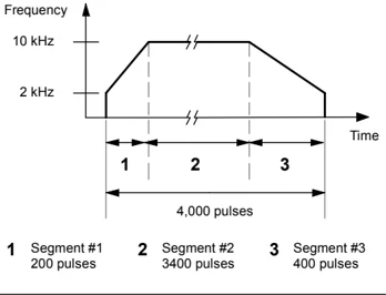
Figure 6-30 Frequency/Time Diagram
For this example: The starting and final pulse frequency is 2 kHz, the maximum pulse frequency is 10 kHz, and 4000 pulses are required to achieve the desired number of motor revolutions. Since the values for the profile table are expressed in terms of period (cycle time) instead of frequency, you must convert the given frequency values into cycle time values. Therefore, the starting (initial) and final (ending) cycle time is 500 \mus, and the cycle time corresponding to the maximum frequency is 100 \mus. During the acceleration portion of the output profile, the maximum pulse frequency should be reached in approximately 200 pulses. The deceleration portion of the profile should be completed in approximately 400 pulses.
You can use the following formula to determine the delta cycle time value for a given segment that the PTO/PWM generator uses to adjust the cycle time of each pulse:
Delta cycle time for a segment = |End_CT_seg - Init_CT_seg| / Quantity_seg
where: End_CT_seg = Ending cycle time for this segment Init_CT_seg = Initial cycle time for this segment $Quantity_{seg}$ = Quantity of pulses in this segment
Using this formula to calculate the delta cycle time values for the sample application:
Segment 1 (acceleration): Delta cycle time = -2
Segment 2 (constant speed): Delta cycle time = 0
Segment 3 (deceleration): Delta cycle time = 1
Table 6-38 lists the values for generating the example waveform (assumes that the profile table is located in V memory, starting at V500). You can include instructions in your program to load these values into V memory, or you can define the values of the profile in the data block.
Table 6-38 Profile Table Values \begin{tabular}{|l|l|l|l|} \hline Address & Value & Description & \ \hline VB500 & 3 & Total number of segments & \ \hline VW501 & 500 & Initial cycle time & \multirow{3}{}{Segment 1} \ \cline{1-3} VW503 & -2 & Initial delta cycle time & \ \cline{1-3} VD505 & 200 & Number of pulses & \ \hline VW509 & 100 & Initial cycle time & \multirow{3}{}{Segment 2} \ \cline{1-3} VW511 & 0 & Delta cycle time & \ \cline{1-3} VD513 & 3400 & Number of pulses & \ \hline VW517 & 100 & Initial cycle time & \multirow{3}{*}{Segment 3} \ \cline{1-3} VW519 & 1 & Delta cycle time & \ \cline{1-3} VD521 & 400 & Number of pulses & \ \hline \end{tabular}
138
S7-200 Instruction Set Chapter 6
In order to determine if the transitions between waveform segments are acceptable, you need to determine the cycle time of the last pulse in a segment. Unless the delta cycle time is 0, you must calculate the cycle time of the last pulse of a segment, because this value is not specified in the profile. Use the following formula to calculate the cycle time of the last pulse:
Cycle time of the last pulse for a segment = Init_CT${seg}$ + ( Delta${seg}$ * ( Quantity$_{seg}$ - 1 ))
where: Init_CT${seg}$ = Initial cycle time for this segment Delta${seg}$ = Delta cycle time for this segment Quantity$_{seg}$ = Quantity of pulses in this segment
While the simplified example above is useful as an introduction, real applications can require more complicated waveform profiles. Remember that the delta cycle time can be specified only as an integer number of microseconds or milliseconds, and the cycle time modification is performed on each pulse.
The effect of these two items is that calculation of the delta cycle time value for a given segment could require an iterative approach. Some flexibility in the value of the ending cycle time or the number of pulses for a given segment might be required.
The duration of a given profile segment can be useful in the process of determining correct profile table values. Use the following formula to calculate the length of time for completing a given profile segment:
Duration of segment = Quantity${seg} * ( Init_CT + ( ( Delta{seg}$/2 ) * ( Quantity$_{seg}$ - 1 ) ) )
where: Quantity${seg}$ = Quantity of pulses in this segment Init_CT${seg}$ = Initial cycle time for this segment Delta$_{seg}$ = Delta cycle time for this segment
139
Math Instructions
Add, Subtract, Multiply, and Divide Instructions
Add
IN1 + IN2 = OUT
FBD
IN1 + OUT = OUT
Subtract
IN1 - IN2 = OUT
OUT - IN1 = OUT
LAD and STL
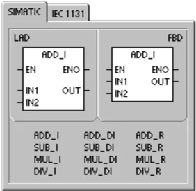
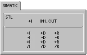
The Add Integer (+I) or Subtract Integer (–I) instructions add or subtract two 16-bit integers to produce a 16-bit result. The Add Double Integer (+D) or Subtract Double Integer (–D) instructions add or subtract two 32-bit integers to produce a 32-bit result. The Add Real (+R) and Subtract Real (–R) instructions add or subtract two 32-bit real numbers to produce a 32-bit real number result.
Multiply
IN1 * IN2 = OUT
FBD
IN1 * OUT = OUT
Divide
IN1 / IN2 = OUT
OUT / IN1 = OUT
LAD and STL
The Multiply Integer (*I) or Divide Integer (/I) instructions multiply or divide two 16-bit integers to produce a 16-bit result. (For division, no remainder is kept.) The Multiply Double Integer (*D) or Divide Double Integer (/D) instructions multiply or divide two 32-bit integers to produce a 32-bit result. (For division, no remainder is kept.) The Multiply Real (*R) or Divide Real (/R) instructions multiply or divide two 32-bit real numbers to produce a 32-bit real number result.
SM Bits and ENO
SM1.1 indicates overflow errors and illegal values. If SM1.1 is set, then the status of SM1.0 and SM1.2 is not valid and the original input operands are not altered. If SM1.1 and SM1.3 are not set, then the math operation has completed with a valid result and SM1.0 and SM1.2 contain valid status. If SM1.3 is set during a divide operation, then the other math status bits are left unchanged.
Error conditions that set ENO = 0
- SM1.1 (overflow)
- SM1.3 (divide by zero)
- 0006 (indirect address)
Special Memory bits affected
- SM1.0 (zero)
- SM1.1 (overflow, illegal value generated during the operation, or illegal input parameter found)
- SM1.2 (negative)
- SM1.3 (divide by zero)
Table 6-39 Valid Operands for Add, Subtract, Multiply, and Divide Instructions
| Inputs/Outputs | Data Types | Operands |
|---|---|---|
| IN1, IN2 | INT | IW, QW, VW, MW, SMW, SW, T, C, LW, AC, AIW, *VD, *AC, *LD, Constant |
| DINT | ID, QD, VD, MD, SMD, SD, LD, AC, HC, *VD, *LD, *AC, Constant | |
| REAL | ID, QD, VD, MD, SMD, SD, LD, AC, *VD, *LD, *AC, Constant | |
| OUT | INT | IW, QW, VW, MW, SMW, SW, LW, T, C, AC, *VD, *AC, *LD |
| DINT, REAL | ID, QD, VD, MD, SMD, SD, LD, AC, *VD, *LD, *AC |
Real (or floating-point) numbers are represented in the format described in the ANSI/IEEE 754–1985 standard (single-precision). Refer to that standard for more information.
S7-200 Instruction Set Chapter 6
Example: Integer Math Instructions
Network 1
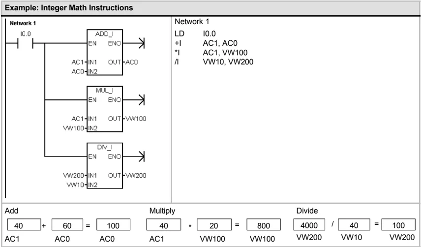
Network 1
LD I0.0 +I AC1, AC0 *I AC1, VW100 /I VW10, VW200
Add
| 40 | + | 60 | = | 100 |
|---|---|---|---|---|
| AC1 | AC0 | AC0 |
Multiply
| 40 | * | 20 | = | 800 |
|---|---|---|---|---|
| AC1 | VW100 | VW100 |
Divide
| 4000 | / | 40 | = | 100 |
|---|---|---|---|---|
| VW200 | VW10 | VW200 |
Example: Real Math Instructions
Network 1
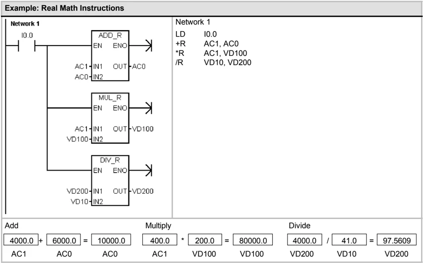
Network 1
LD I0.0 +R AC1, AC0 *R AC1, VD100 /R VD10, VD200
Add
| 4000.0 | + | 6000.0 | = | 10000.0 |
|---|---|---|---|---|
| AC1 | AC0 | AC0 |
Multiply
| 400.0 | * | 200.0 | = | 80000.0 |
|---|---|---|---|---|
| AC1 | VD100 | VD100 |
Divide
| 4000.0 | / | 41.0 | = | 97.5609 |
|---|---|---|---|---|
| VD200 | VD10 | VD200 |
141
Multiply Integer to Double Integer and Divide Integer with Remainder
Multiply Integer to Double Integer
IN1 * IN2 = OUT LAD and FBD
IN1 * OUT = OUT STL
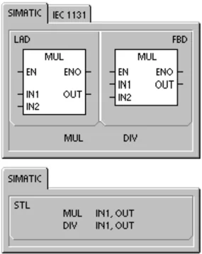
The Multiply Integer to Double Integer instruction (MUL) multiplies two 16-bit integers and produces a 32-bit product. In the STL MUL instruction, the least-significant word (16 bits) of the 32-bit OUT is used as one of the factors.
Divide Integer with Remainder
IN1 / IN2 = OUT LAD and FBD
OUT / IN1 = OUT STL
The Divide Integer with Remainder instruction (DIV) divides two 16-bit integers and produces a 32-bit result consisting of a 16-bit remainder (the most-significant word) and a 16-bit quotient (the least-significant word).
In STL, the least-significant word (16 bits) of the 32-bit OUT is used as the dividend.
SM Bits and ENO
For both of the instructions on this page, Special Memory (SM) bits indicate errors and illegal values. If SM1.3 (divide by zero) is set during a divide operation, then the other math status bits are left unchanged. Otherwise, all supported math status bits contain valid status upon completion of the math operation.
Error conditions that set ENO = 0
- SM1.1 (overflow)
- SM1.3 (divide by zero)
- 0006 (indirect address)
Special Memory bits affected
- SM1.0 (zero)
- SM1.1 (overflow)
- SM1.2 (negative)
- SM1.3 (divide by zero)
Table 6-40 Valid Operands for Multiply Integer to Double Integer and Divide Integer with Remainder
| Inputs/Outputs | Data Types | Operands |
|---|---|---|
| IN1, IN2 | INT | IW, QW, VW, MW, SMW, SW, T, C, LW, AC, AIW, *VD, *LD, *AC, Constant |
| OUT | DINT | ID, QD, VD, MD, SMD, SD, LD, AC, *VD, *LD, *AC |
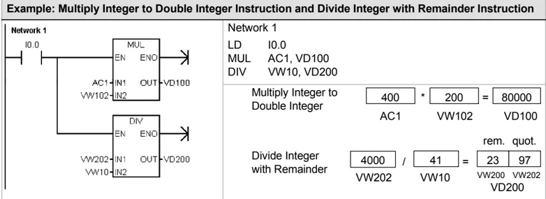
Example: Multiply Integer to Double Integer Instruction and Divide Integer with Remainder Instruction
Note: VD100 contains: VW100 and VW102, and VD200 contains: VW200 and VW202.
Numeric Functions Instructions
Sine, Cosine, and Tangent
The Sine (SIN), Cosine (COS), and Tangent (TAN) instructions evaluate the trigonometric function of the angle value IN and place the result in OUT. The input angle value is in radians.
$$ \text{SIN (IN) = OUT} \quad \text{COS (IN) = OUT} \quad \text{TAN (IN) = OUT} $$
To convert an angle from degrees to radians: Use the MUL_R (*R) instruction to multiply the angle in degrees by 1.745329E-2 (approximately by \pi/180).
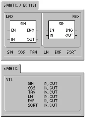
Natural Logarithm and Natural Exponential
The Natural Logarithm instruction (LN) performs the natural logarithm of the value in IN and places the result in OUT.
The Natural Exponential instruction (EXP) performs the exponential operation of e raised to the power of the value in IN and places the result in OUT.
$$ \text{LN (IN) = OUT} \quad \text{EXP (IN)= OUT} $$
To obtain the base 10 logarithm from the natural logarithm: Divide the natural logarithm by 2.302585 (approximately the natural logarithm of 10).
To raise any real number to the power of another real number, including fractional exponents: Combine the Natural Exponential instruction with the Natural Logarithm instruction. For example, to raise X to the Y power, enter the following instruction: EXP (Y * LN (X)).
Square Root
The Square Root instruction (SQRT) takes the square root of a real number (IN) and produces a real number result OUT.
$$ \text{SQRT (IN)= OUT} $$
To obtain other roots: 5 cubed = $5^3$ = EXP(3*LN(5)) = 125 The cube root of 125 = $125^{(1/3)}$ = EXP((1/3)LN(125))= 5 The square root of 5 cubed = $5^{(3/2)}$ = EXP(3/2LN(5)) = 11.18034
SM Bits and ENO for the Numeric Functions Instructions
For all of the instructions that are described on this page, SM1.1 is used to indicate overflow errors and illegal values. If SM1.1 is set, then the status of SM1.0 and SM1.2 is not valid and the original input operands are not altered. If SM1.1 is not set, then the math operation has completed with a valid result and SM1.0 and SM1.2 contain valid status.
Error conditions that set ENO = 0
- SM1.1 (overflow)
- 0006 (indirect address)
Special Memory bits affected
- SM1.0 (zero)
- SM1.1 (overflow)
- SM1.2 (negative)
Table 6-41 Valid Operands for Numeric Functions \begin{tabular}{|l|l|l|} \hline Inputs/Outputs & Data Types & Operands \ \hline IN & REAL & ID, QD, VD, MD, SMD, SD, LD, AC, *VD, *LD, *AC, Constant \ \hline OUT & REAL & ID, QD, VD, MD, SMD, SD, LD, AC, *VD, *LD, *AC \ \hline \end{tabular}
Real (or floating-point) numbers are represented in the format described in the ANSI/IEEE 754-1985 standard (single-precision). Refer to that standard for more information.
Increment and Decrement Instructions
Increment
IN + 1 = OUT LAD and FBD OUT + 1 = OUT STL
Decrement
IN - 1 = OUT LAD and FBD OUT - 1 = OUT STL
The Increment and Decrement instructions add or subtract 1 to or from the input IN and place the result into the variable OUT.
Increment Byte (INCB) and Decrement Byte (DECB) operations are unsigned.
Increment Word (INCW) and Decrement Word (DECW) operations are signed.
Increment Double Word (INCD) and Decrement Double Word (DECD) operations are signed.
Error conditions that set ENO = 0:
- SM1.1 (overflow)
- 0006 (indirect address)
Special Memory bits affected:
- SM1.0 (zero)
- SM1.1 (overflow)
- SM1.2 (negative) for Word and Double Word operations
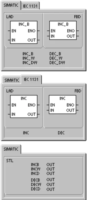
Table 6-42 Valid Operands for the Increment and Decrement Instructions \begin{tabular}{|l|l|l|} \hline Inputs/Outputs & Data Types & Operands \ \hline IN & BYTE & IB, QB, VB, MB, SMB, SB, LB, AC, *VD, *LD, *AC, Constant \ & INT & IW, QW, VW, MW, SMW, SW, T, C, LW, AC, AIW, *VD, *LD, *AC, Constant \ & DINT & ID, QD, VD, MD, SMD, SD, LD, AC, HC, *VD, *LD, *AC, Constant \ \hline OUT & BYTE & IB, QB, VB, MB, SMB, SB, LB, AC, *VD, *AC, *LD \ & INT & IW, QW, VW, MW, SMW, SW, T, C, LW, AC, *VD, *LD, *AC \ & DINT & ID, QD, VD, MD, SMD, SD, LD, AC, *VD, *LD, *AC \ \hline \end{tabular}
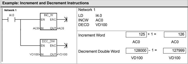
Example: Increment and Decrement Instructions
144
Proportional/Integral/Derivative (PID) Loop Instruction
The PID Loop instruction (PID) executes a PID loop calculation on the referenced LOOP based on the input and configuration information in Table (TBL).
Error conditions that set ENO = 0:
- SM1.1 (overflow)
- 0006 (indirect address)
Special Memory bits affected:
- SM1.1 (overflow)
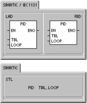
The PID loop instruction (Proportional, Integral, Derivative Loop) is provided to perform the PID calculation. The top of the logic stack (TOS) must be ON (power flow) to enable the PID calculation. The instruction has two operands: a TABLE address which is the starting address of the loop table and a LOOP number which is a constant from 0 to 7.
Eight PID instructions can be used in a program. If two or more PID instructions are used with the same loop number (even if they have different table addresses), the PID calculations will interfere with one another and the output will be unpredictable.
The loop table stores nine parameters used for controlling and monitoring the loop operation and includes the current and previous value of the process variable, the setpoint, output, gain, sample time, integral time (reset), derivative time (rate), and the integral sum (bias).
To perform the PID calculation at the desired sample rate, the PID instruction must be executed either from within a timed interrupt routine or from within the main program at a rate controlled by a timer. The sample time must be supplied as an input to the PID instruction via the loop table.
Auto-Tune capability has been incorporated into the PID instruction. Refer to Chapter 15 for a detailed description of auto-tuning. The PID Tuning Control Panel only works with PID loops created by the PID wizard..
Table 6-43 Valid Operands for the PID Loop Instruction \begin{tabular}{|l|l|l|} \hline Inputs/Outputs & Data Types & Operands \ \hline TBL & BYTE & VB \ \hline LOOP & BYTE & Constant (0 to 7) \ \hline \end{tabular}
Instruction Wizard STEP 7-Micro/WIN offers the PID Wizard to guide you in defining a PID algorithm for a closed-loop control process. Select the Tools > Instruction Wizard menu command and then select PID from the Instruction Wizard window.
Tip The setpoint of the low range and the setpoint of the high range should correspond to the process variable low range and high range.
Understanding the PID Algorithm
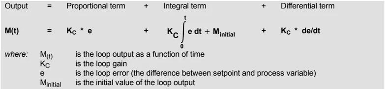
In steady state operation, a PID controller regulates the value of the output so as to drive the error (e) to zero. A measure of the error is given by the difference between the setpoint (S P) (the desired operating point) and the process variable (PV) (the actual operating point). The principle of PID control is based upon the following equation that expresses the output, M(t), as a function of a proportional term, an integral term, and a differential term:
| Output | = | Proportional term | + | Integral term | + | Differential term |
|---|---|---|---|---|---|---|
| M(t) | = | KC * e | + | KC ∫0t e dt + Minitial | + | KC * de/dt |
where:
- M(t) is the loop output as a function of time
- KC is the loop gain
- e is the loop error (the difference between setpoint and process variable)
- Minitial is the initial value of the loop output
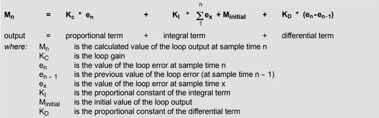
In order to implement this control function in a digital computer, the continuous function must be quantized into periodic samples of the error value with subsequent calculation of the output. The corresponding equation that is the basis for the digital computer solution is:
| Mn | = | KC * en | + | KI * Σ1n ex + Minitial | + | KD * (en-en-1) |
|---|---|---|---|---|---|---|
| output | = | proportional term | + | integral term | + | differential term |
where:
- Mn is the calculated value of the loop output at sample time n
- KC is the loop gain
- en is the value of the loop error at sample time n
- en - 1 is the previous value of the loop error (at sample time n - 1)
- ex is the value of the loop error at sample time x
- KI is the proportional constant of the integral term
- Minitial is the initial value of the loop output
- KD is the proportional constant of the differential term
From this equation, the integral term is shown to be a function of all the error terms from the first sample to the current sample. The differential term is a function of the current sample and the previous sample, while the proportional term is only a function of the current sample. In a digital computer, it is not practical to store all samples of the error term, nor is it necessary.
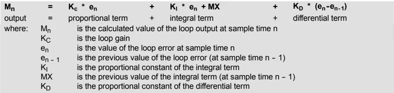
Since the digital computer must calculate the output value each time the error is sampled beginning with the first sample, it is only necessary to store the previous value of the error and the previous value of the integral term. As a result of the repetitive nature of the digital computer solution, a simplification in the equation that must be solved at any sample time can be made. The simplified equation is:
| Mn | = | KC * en | + | KI * en + MX | + | KD * (en-en-1) |
|---|---|---|---|---|---|---|
| output | = | proportional term | + | integral term | + | differential term |
where:
- Mn is the calculated value of the loop output at sample time n
- KC is the loop gain
- en is the value of the loop error at sample time n
- en - 1 is the previous value of the loop error (at sample time n - 1)
- KI is the proportional constant of the integral term
- MX is the previous value of the integral term (at sample time n - 1)
- KD is the proportional constant of the differential term
The S 7-200 uses a modified form of the above simplified equation when calculating the loop output value. This modified equation is:
| Mn | = | MPn | + | MIn | + | MDn |
|---|---|---|---|---|---|---|
| output | = | proportional term | + | integral term | + | differential term |
where:
- Mn is the calculated value of the loop output at sample time n
- MPn is the value of the proportional term of the loop output at sample time n
- MIn is the value of the integral term of the loop output at sample time n
- MDn is the value of the differential term of the loop output at sample time n
Understanding the Proportional Term of the PID Equation
The proportional term MP is the product of the gain (KC), which controls the sensitivity of the output calculation, and the error (e), which is the difference between the setpoint (SP) and the process variable (PV) at a given sample time. The equation for the proportional term as solved by the S 7-200 is:
| MPn | = | KC | * | (SPn - PVn) |
|---|
where:
- MPn is the value of the proportional term of the loop output at sample time n
- KC is the loop gain
- SPn is the value of the setpoint at sample time n
- PVn is the value of the process variable at sample time n
Understanding the Integral Term of the PID Equation
The integral term MI is proportional to the sum of the error over time. The equation for the integral term as solved by the S 7-200 is:
| MIn | = | KC | * | TS | / | TI | * | (SPn - PVn) | + | MX |
|---|
where:
- MIn is the value of the integral term of the loop output at sample time n
- KC is the loop gain
- TS is the loop sample time
- TI is the integration period of the loop (also called the integral time or reset)
- SPn is the value of the setpoint at sample time n
- PVn is the value of the process variable at sample time n
- MX is the value of the integral term at sample time n - 1 (also called the integral sum or the bias)
The integral sum or bias (MX) is the running sum of all previous values of the integral term. After each calculation of MIn, the bias is updated with the value of MIn which might be adjusted or clamped (see the section “Variables and Ranges” for details). The initial value of the bias is typically set to the output value (Minitial) just prior to the first loop output calculation. Several constants are also part of the integral term, the gain (KC), the sample time (TS), which is the cycle time at which the PID loop recalculates the output value, and the integral time or reset (TI), which is a time used to control the influence of the integral term in the output calculation.
Understanding the Differential Term of the PID Equation The differential term MD is proportional to the change in the error. The S7-200 uses the following equation for the differential term:
$$MD_n = K_C * T_D / T_S * ((SP_n - PV_n) - (SP_{n-1} - PV_{n-1}))$$
To avoid step changes or bumps in the output due to derivative action on setpoint changes, this equation is modified to assume that the setpoint is a constant ($SP_n = SP_{n-1}$). This results in the calculation of the change in the process variable instead of the change in the error as shown:
$$MD_n = K_C * T_D / T_S * (SP_n - PV_n - SP_n + PV_{n-1})$$
or just:
$$MD_n = K_C * T_D / T_S * (PV_{n-1} - PV_n)$$
where: $MD_n$ is the value of the differential term of the loop output at sample time n $K_C$ is the loop gain $T_S$ is the loop sample time $T_D$ is the differentiation period of the loop (also called the derivative time or rate) $SP_n$ is the value of the setpoint at sample time n $SP_{n-1}$ is the value of the setpoint at sample time n-1 $PV_n$ is the value of the process variable at sample time n $PV_{n-1}$ is the value of the process variable at sample time n-1
The process variable rather than the error must be saved for use in the next calculation of the differential term. At the time of the first sample, the value of $PV_{n-1}$ is initialized to be equal to $PV_n$.
Selecting the Type of Loop Control In many control systems, it might be necessary to employ only one or two methods of loop control. For example, only proportional control or proportional and integral control might be required. The selection of the type of loop control desired is made by setting the value of the constant parameters.
If you do not want integral action (no "I" in the PID calculation), then a value of infinity "INF", should be specified for the integral time (reset). Even with no integral action, the value of the integral term might not be zero, due to the initial value of the integral sum MX.
If you do not want derivative action (no "D" in the PID calculation), then a value of 0.0 should be specified for the derivative time (rate).
If you do not want proportional action (no "P" in the PID calculation) and you want I or ID control, then a value of 0.0 should be specified for the gain. Since the loop gain is a factor in the equations for calculating the integral and differential terms, setting a value of 0.0 for the loop gain will result in a value of 1.0 being used for the loop gain in the calculation of the integral and differential terms.
Converting and Normalizing the Loop Inputs A loop has two input variables, the setpoint and the process variable. The setpoint is generally a fixed value such as the speed setting on the cruise control in your automobile. The process variable is a value that is related to loop output and therefore measures the effect that the loop output has on the controlled system. In the example of the cruise control, the process variable would be a tachometer input that measures the rotational speed of the tires.
148
S7-200 Instruction Set Chapter 6
Both the setpoint and the process variable are real world values whose magnitude, range, and engineering units could be different. Before these real world values can be operated upon by the PID instruction, the values must be converted to normalized, floating-point representations.
The first step is to convert the real world value from a 16-bit integer value to a floating-point or real number value. The following instruction sequence is provided to show how to convert from an integer value to a real number.
| ITD | AIW0, AC0 | //Convert an input value to a double word |
|---|---|---|
| DTR | AC0, AC0 | //Convert the 32-bit integer to a real number |
The next step is to convert the real number value representation of the real world value to a normalized value between 0.0 and 1.0. The following equation is used to normalize either the setpoint or process variable value:
RNorm = ((RRaw / Span) + Offset)
where: RNorm is the normalized, real number value representation of the real world value
RRaw is the un-normalized or raw, real number value representation of the real world value
Offset is 0.0 for unipolar values
is 0.5 for bipolar values
Span is the maximum possible value minus the minimum possible value:
= 32,000 for unipolar values (typical)
= 64,000 for bipolar values (typical)
The following instruction sequence shows how to normalize the bipolar value in AC0 (whose span is 64,000) as a continuation of the previous instruction sequence:
| /R | 64000.0, AC0 | //Normalize the value in the accumulator |
|---|---|---|
| +R | 0.5, AC0 | //Offset the value to the range from 0.0 to 1.0 |
| MOVR | AC0, VD100 | //Store the normalized value in the loop TABLE |
Converting the Loop Output to a Scaled Integer Value
The loop output is the control variable, such as the throttle setting of the cruise control on an automobile. The loop output is a normalized, real number value between 0.0 and 1.0. Before the loop output can be used to drive an analog output, the loop output must be converted to a 16-bit, scaled integer value. This process is the reverse of converting the PV and SP to a normalized value. The first step is to convert the loop output to a scaled, real number value using the formula given below:
RScal = (Mn - Offset) * Span
where: RScal is the scaled, real number value of the loop output
Mn is the normalized, real number value of the loop output
Offset is 0.0 for unipolar values
is 0.5 for bipolar values
Span is the maximum possible value minus the minimum possible value
= 32,000 for unipolar values (typical)
= 64,000 for bipolar values (typical)
149
The following instruction sequence shows how to scale the loop output:
| MOVR VD108, AC0 | //Moves the loop output to the accumulator |
|---|---|
| -R 0.5, AC0 | //Include this statement only if the value is bipolar |
| *R 64000.0, AC0 | //Scales the value in the accumulator |
Next, the scaled, real number value representing the loop output must be converted to a 16-bit integer. The following instruction sequence shows how to do this conversion:
| ROUND AC0, AC0 | //Converts the real number to a 32-bit integer |
|---|---|
| DTI AC0, LW0 | //Converts the value to a 16-bit integer |
| MOVW LW0, AQW0 | //Writes the value to the analog output |
Forward- or Reverse-Acting Loops
The loop is forward-acting if the gain is positive and reverse-acting if the gain is negative. (For I or ID control, where the gain value is 0.0, specifying positive values for integral and derivative time will result in a forward-acting loop, and specifying negative values will result in a reverse-acting loop.)
Variables and Ranges
The process variable and setpoint are inputs to the PID calculation. Therefore the loop table fields for these variables are read but not altered by the PID instruction.
The output value is generated by the PID calculation, so the output value field in the loop table is updated at the completion of each PID calculation. The output value is clamped between 0.0 and 1.0. The output value field can be used as an input by the user to specify an initial output value when making the transition from manual control to PID instruction (auto) control of the output. (See the discussion in the “Modes” section below).
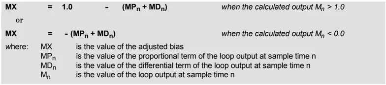
If integral control is being used, then the bias value is updated by the PID calculation and the updated value is used as an input in the next PID calculation. When the calculated output value goes out of range (output would be less than 0.0 or greater than 1.0), the bias is adjusted according to the following formulas:
| MX = 1.0 - (MPₙ + MDₙ) | when the calculated output Mₙ > 1.0 |
|---|---|
| or | |
| MX = - (MPₙ + MDₙ) | when the calculated output Mₙ < 0.0 |
where:
MX is the value of the adjusted bias
MPₙ is the value of the proportional term of the loop output at sample time n
MDₙ is the value of the differential term of the loop output at sample time n
Mₙ is the value of the loop output at sample time n
By adjusting the bias as described, an improvement in system responsiveness is achieved once the calculated output comes back into the proper range. The calculated bias is also clamped between 0.0 and 1.0 and then is written to the bias field of the loop table at the completion of each PID calculation. The value stored in the loop table is used in the next PID calculation.
The bias value in the loop table can be modified by the user prior to execution of the PID instruction in order to address bias value problems in certain application situations. Care must be taken when manually adjusting the bias, and any bias value written into the loop table must be a real number between 0.0 and 1.0.
A comparison value of the process variable is maintained in the loop table for use in the derivative action part of the PID calculation. You should not modify this value.
150
S7-200 Instruction Set Chapter 6
Modes
There is no built-in mode control for S7-200 PID loops. The PID calculation is performed only when power flows to the PID box. Therefore, "automatic" or "auto" mode exists when the PID calculation is performed cyclically. "Manual" mode exists when the PID calculation is not performed.
The PID instruction has a power-flow history bit, similar to a counter instruction. The instruction uses this history bit to detect a 0-to-1 power-flow transition. When the power-flow transition is detected, it will cause the instruction to perform a series of actions to provide a bumpless change from manual control to auto control. In order for change to auto mode control to be bumpless, the value of the output as set by the manual control must be supplied as an input to the PID instruction (written to the loop table entry for $M_n$) before switching to auto control. The PID instruction performs the following actions to values in the loop table to ensure a bumpless change from manual to auto control when a 0-to-1 power-flow transition is detected:
\square Sets setpoint ($SP_n$) = process variable ($PV_n$)
\square Sets old process variable ($PV_{n-1}$) = process variable ($PV_n$)
\square Sets bias ($MX$) = output value ($M_n$)
The default state of the PID history bits is "set" and that state is established at startup and on every STOP-to-RUN mode transition of the controller. If power flows to the PID box the first time that it is executed after entering RUN mode, then no power-flow transition is detected and the bumpless mode change actions are not performed.
Alarm Checking and Special Operations
The PID instruction is a simple but powerful instruction that performs the PID calculation. If other processing is required such as alarm checking or special calculations on loop variables, these must be implemented using the basic instructions supported by the S7-200.
Error Conditions
When it is time to compile, the CPU will generate a compile error (range error) and the compilation will fail if the loop table start address or PID loop number operands specified in the instruction are out of range.
Certain loop table input values are not range checked by the PID instruction. You must take care to ensure that the process variable and setpoint (as well as the bias and previous process variable if used as inputs) are real numbers between 0.0 and 1.0.
If any error is encountered while performing the mathematical operations of the PID calculation, then SM1.1 (overflow or illegal value) is set and execution of the PID instruction is terminated. (Update of the output values in the loop table could be incomplete, so you should disregard these values and correct the input value causing the mathematical error before the next execution of the loop's PID instruction.)
Loop Table
The loop table is 80 bytes long and has the format shown in Table 6-44.
Table 6-44 Loop Table
| Offset | Field | Format | Type | Description |
|---|---|---|---|---|
| 0 | Process variable (PVₙ) | REAL | In | Contains the process variable, which must be scaled between 0.0 and 1.0. |
| 4 | Setpoint (SPₙ) | REAL | In | Contains the setpoint, which must be scaled between 0.0 and 1.0. |
| 8 | Output (Mₙ) | REAL | In/Out | Contains the calculated output, scaled between 0.0 and 1.0. |
| 12 | Gain (Kc) | REAL | In | Contains the gain, which is a proportional constant. Can be a positive or negative number. |
| 16 | Sample time (Tₛ) | REAL | In | Contains the sample time, in seconds. Must be a positive number. |
| 20 | Integral time or reset (Tᵢ) | REAL | In | Contains the integral time or reset, in minutes. Must be a positive number. |
| 24 | Derivative time or rate (Tᴅ) | REAL | In | Contains the derivative time or rate, in minutes. Must be a positive number. |
| 28 | Bias (MX) | REAL | In/Out | Contains the bias or integral sum value between 0.0 and 1.0. |
| 32 | Previous process variable (PVₙ₋₁) | REAL | In/Out | Contains the value of the process variable stored from the last execution of the PID instruction. |
| 36 to 79 | Reserved for auto-tuning variables. Refer to Table 15-1 for details. |
Interrupt Instructions
Enable Interrupt and Disable Interrupt
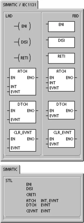
The Enable Interrupt instruction (ENI) globally enables processing of all attached interrupt events. The Disable Interrupt instruction (DISI) globally disables processing of all interrupt events.
When you make the transition to RUN mode, interrupts are initially disabled. In RUN mode, you can enable interrupt processing by executing the Enable Interrupt instruction. Executing the Disable Interrupt instruction inhibits the processing of interrupts; however, active interrupt events will continue to be queued.
Error conditions that set ENO = 0:
- 0004 (attempted execution of ENI, DISI, or HDEF instructions in an interrupt routine)
Conditional Return from Interrupt
The Conditional Return from Interrupt instruction (CRETI) can be used to return from an interrupt, based upon the condition of the preceding logic.
Attach Interrupt
The Attach Interrupt instruction (ATCH) associates an interrupt event EVNT with an interrupt routine number INT and enables the interrupt event.
Error conditions that set ENO = 0:
- 0002 (conflicting assignment of inputs to an HSC)
Detach Interrupt
The Detach Interrupt instruction (DTCH) disassociates an interrupt event EVNT from all interrupt routines and disables the interrupt event.
Clear Interrupt Event
The Clear Interrupt Event instruction removes all interrupt events of type EVNT from the interrupt queue. Use this instruction to clear the interrupt queue of unwanted interrupt events. If this instruction is being used to clear out spurious interrupt events, you should detach the event before clearing the events from the queue. Otherwise new events will be added to the queue after the clear event instruction has been executed.
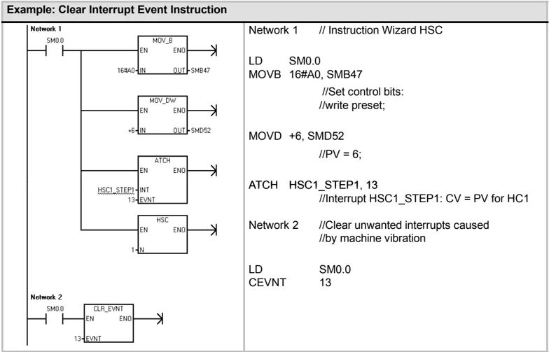
The example shows a high-speed counter in quadrature mode using the CLR_EVNT instruction to remove interrupts. If a light chopper stepper sensor was stopped in a position that is on the edge of a light to dark transition, then small machine vibrations could generate unwanted interrupts before the new PV can be loaded.
SIMATIC STL ENI DISI <CRETI ATCH INT_EVNT DTCH EVNT <EVNT EVNT
Table 6-45 Valid Operands for the Interrupt Instructions
Operation of the Attach Interrupt and Detach Interrupt Instructions
Before an interrupt routine can be invoked, an association must be established between the interrupt event and the program segment that you want to execute when the event occurs. Use the Attach Interrupt instruction to associate an interrupt event (specified by the interrupt event number) and the program segment (specified by an interrupt routine number). You can attach multiple interrupt events to one interrupt routine, but one event cannot be concurrently attached to multiple interrupt routines.
When you attach an interrupt event to an interrupt routine, that interrupt is automatically enabled. If you disable all interrupts using the global disable interrupt instruction, each occurrence of the interrupt event is queued until interrupts are re-enabled, using the global enable interrupt instruction, or the interrupt queue overflows.
You can disable individual interrupt events by breaking the association between the interrupt event and the interrupt routine with the Detach Interrupt instruction. The Detach Interrupt instruction returns the interrupt to an inactive or ignored state. Table 6-46 lists the different types of interrupt events.
Table 6-46 Interrupt Events
| Event | Description | CPU 221 CPU 222 | CPU 224 | CPU 224XP CPU 226 |
|---|---|---|---|---|
| 0 | I0.0 Rising edge | Y | Y | Y |
| 1 | I0.0 Falling edge | Y | Y | Y |
| 2 | I0.1 Rising edge | Y | Y | Y |
| 3 | I0.1 Falling edge | Y | Y | Y |
| 4 | I0.2 Rising edge | Y | Y | Y |
| 5 | I0.2 Falling edge | Y | Y | Y |
| 6 | I0.3 Rising edge | Y | Y | Y |
| 7 | I0.3 Falling edge | Y | Y | Y |
| 8 | Port 0 Receive character | Y | Y | Y |
| 9 | Port 0 Transmit complete | Y | Y | Y |
| 10 | Timed interrupt 0 SMB34 | Y | Y | Y |
| 11 | Timed interrupt 1 SMB35 | Y | Y | Y |
| 12 | HSC 0 CV=PV (current value = preset value) | Y | Y | Y |
| 13 | HSC 1 CV=PV (current value = preset value) | Y | Y | |
| 14 | HSC 1 Direction changed | Y | Y | |
| 15 | HSC 1 External reset | Y | Y | |
| 16 | HSC 2 CV=PV (current value = preset value) | Y | Y | |
| 17 | HSC 2 Direction changed | Y | Y | |
| 18 | HSC 2 External reset | Y | Y | |
| 19 | PLS 0 PTO pulse count complete interrupt | Y | Y | Y |
| 20 | PLS 1 PTO pulse count complete interrupt | Y | Y | Y |
| 21 | Timer T32 CT=PT interrupt | Y | Y | Y |
S7-200 Instruction Set Chapter 6
Table 6-46 Interrupt Events, continued
Understanding How the S7-200 Processes Interrupt Routines
The interrupt routine is executed in response to an associated internal or external event. Once the last instruction of the interrupt routine has been executed, control is returned to the main program. You can exit the routine by executing a Conditional Return from Interrupt instruction (CRETI). Table 6-47 emphasizes some guidelines and restrictions for using interrupt routines in your program.
Table 6-47 Guidelines and Restrictions for Using Interrupt Routines
System Support for Interrupts
Because contact, coil, and accumulator logic can be affected by interrupts, the system saves and reloads the logic stack, accumulator registers, and the special memory bits (SM) that indicate the status of accumulator and instruction operations. This avoids disruption to the main user program caused by branching to and from an interrupt routine.
Sharing Data Between the Main Program and Interrupt Routines
You can share data between the main program and one or more interrupt routines. Because it is not possible to predict when the S7-200 might generate an interrupt, it is desirable to limit the number of variables that are used by both the interrupt routine and elsewhere in the program. Problems with the consistency of shared data can result due to the actions of interrupt routines when the execution of instructions in your main program is interrupted by interrupt events. Use the local variable table of the interrupt routine to ensure that your interrupt routine uses only the temporary memory and does not overwrite data used somewhere else in your program.
There are a number of programming techniques you can use to ensure that data is correctly shared between your main program and interrupt routines. These techniques either restrict the way access is made to shared memory locations or prevent interruption of instruction sequences using shared memory locations.
For an STL program that is sharing a single variable: If the shared data is a single byte, word, or double word variable and your program is written in STL, then correct shared access can be ensured by storing the intermediate values from operations on shared data only in non-shared memory locations or accumulators.
For a LAD program that is sharing a single variable: If the shared data is a single byte, word, or double word variable and your program is written in LAD, then correct shared access can be ensured by establishing the convention that access to shared memory locations be made using only Move instructions (MOVB, MOVW, MOVD, MOVR). While many LAD instructions are composed of interruptible sequences of STL instructions, these Move instructions are composed of a single STL instruction whose execution cannot be affected by interrupt events.
For an STL or LAD program that is sharing multiple variables: If the shared data is composed of a number of related bytes, words, or double words, then the interrupt disable/enable instructions (DISI and ENI) can be used to control interrupt routine execution. At the point in your main program where operations on shared memory locations are to begin, disable the interrupts. Once all actions affecting the shared locations are complete, re-enable the interrupts. During the time that interrupts are disabled, interrupt routines cannot be executed and therefore cannot access shared memory locations; however, this approach can result in delayed response to interrupt events.
Calling Subroutines from Interrupt Routines You can call one nesting level of subroutines from an interrupt routine. The accumulators and the logic stack are shared between an interrupt routine and a subroutine that is called.
Types of Interrupts Supported by the S7-200 The S7-200 supports the following types of interrupt routines:
Communications port interrupts: The S7-200 generates events that allow your program to control the communications port.
I/O interrupts: The S7-200 generates events for different changes of state for various I/O. These events allow your program to respond to the high-speed counters, the pulse outputs, or to rising or falling states of the inputs.
Time-based interrupts: The S7-200 generates events that allow your program to react at specific intervals.
Communications Port Interrupts The serial communications port of the S7-200 can be controlled by your program. This mode of operating the communications port is called Freeport mode. In Freeport mode, your program defines the baud rate, bits per character, parity, and protocol. The Receive and Transmit interrupts are available to facilitate your program-controlled communications. Refer to the Transmit and Receive instructions for more information.
I/O Interrupts I/O interrupts include rising/falling edge interrupts, high-speed counter interrupts, and pulse train output interrupts. The S7-200 can generate an interrupt on rising and/or falling edges of an input (either I0.0, I0.1, I0.2, or I0.3). The rising edge and the falling edge events can be captured for each of these input points. These rising/falling edge events can be used to signify a condition that must receive immediate attention when the event happens.
The high-speed counter interrupts allow you to respond to conditions such as the current value reaching the preset value, a change in counting direction that might correspond to a reversal in the direction in which a shaft is turning, or an external reset of the counter. Each of these high-speed counter events allows action to be taken in real time in response to high-speed events that cannot be controlled at programmable logic controller scan speeds.
156
The pulse train output interrupts provide immediate notification of completion of outputting the prescribed number of pulses. A typical use of pulse train outputs is stepper motor control.
You can enable each of the above interrupts by attaching an interrupt routine to the related I/O event.
Time-Based Interrupts
Time-based interrupts include timed interrupts and the timer T32/T96 interrupts. You can specify actions to be taken on a cyclic basis using a timed interrupt. The cycle time is set in 1-ms increments from 1 ms to 255 ms. You must write the cycle time in SMB34 for timed interrupt 0, and in SMB35 for timed interrupt 1.
The timed interrupt event transfers control to the appropriate interrupt routine each time the timer expires. Typically, you use timed interrupts to control the sampling of analog inputs or to execute a PID loop at regular intervals.
A timed interrupt is enabled and timing begins when you attach an interrupt routine to a timed interrupt event. During the attachment, the system captures the cycle time value, so subsequent changes to SMB34 and SMB35 do not affect the cycle time. To change the cycle time, you must modify the cycle time value, and then re-attach the interrupt routine to the timed interrupt event. When the re-attachment occurs, the timed interrupt function clears any accumulated time from the previous attachment and begins timing with the new value.
After being enabled, the timed interrupt runs continuously, executing the attached interrupt routine on each expiration of the specified time interval. If you exit RUN mode or detach the timed interrupt, the timed interrupt is disabled. If the global disable interrupt instruction is executed, timed interrupts continue to occur. Each occurrence of the timed interrupt is queued (until either interrupts are enabled or the queue is full).
The timer T32/T96 interrupts allow timely response to the completion of a specified time interval. These interrupts are only supported for the 1-ms resolution on-delay (TON) and off-delay (TOF) timers T32 and T96. The T32 and T96 timers otherwise behave normally. Once the interrupt is enabled, the attached interrupt routine is executed when the active timer’s current value becomes equal to the preset time value during the normal 1-ms timer update performed in the S7-200. You enable these interrupts by attaching an interrupt routine to the T32/T96 interrupt events.
Interrupt Priority and Queuing
Interrupts are serviced by the S7-200 on a first-come-first-served basis within their respective priority group. Only one user-interrupt routine is ever being executed at any point in time. Once the execution of an interrupt routine begins, the routine is executed to completion. It cannot be pre-empted by another interrupt routine, even by a higher priority routine. Interrupts that occur while another interrupt is being processed are queued for later processing.
Table 6-48 shows the three interrupt queues and the maximum number of interrupts they can store.
Table 6-48 Maximum Number of Entries per Interrupt Queue
| Queue | CPU 221, CPU 222, CPU 224 | CPU 224XP and CPU 226 |
|---|---|---|
| Communications queue | 4 | 8 |
| I/O Interrupt queue | 16 | 16 |
| Timed Interrupt queue | 8 | 8 |
Potentially, more interrupts can occur than the queue can hold. Therefore, queue overflow memory bits (identifying the type of interrupt events that have been lost) are maintained by the system. Table 6-49 shows the interrupt queue overflow bits. You should use these bits only in an interrupt routine because they are reset when the queue is emptied, and control is returned to the main program.
Table 6-50 shows all interrupt events, with their priority and assigned event number.
Table 6-49 Interrupt Queue Overflow Bits
| Description (0 = No Overflow, 1 = Overflow) | SM Bit |
|---|---|
| Communications queue | SM4.0 |
| I/O Interrupt queue | SM4.1 |
| Timed Interrupt queue | SM4.2 |
Table 6-50 Priority Order for Interrupt Events
| Event | Description | Priority Group | Priority in Group |
|---|---|---|---|
| 8 | Port 0 Receive character | Communications Highest Priority | 0 |
| 9 | Port 0 Transmit complete | 0 | |
| 23 | Port 0 Receive message complete | 0 | |
| 24 | Port 1 Receive message complete | 1 | |
| 25 | Port 1 Receive character | 1 | |
| 26 | Port 1 Transmit complete | 1 | |
| 19 | PLS 0 PTO pulse count complete interrupt | Discrete Medium Priority | 0 |
| 20 | PLS 1 PTO pulse count complete interrupt | 1 | |
| 0 | I0.0 Rising edge | 2 | |
| 2 | I0.1 Rising edge | 3 | |
| 4 | I0.2 Rising edge | 4 | |
| 6 | I0.3 Rising edge | 5 | |
| 1 | I0.0 Falling edge | 6 | |
| 3 | I0.1 Falling edge | 7 | |
| 5 | I0.2 Falling edge | 8 | |
| 7 | I0.3 Falling edge | 9 | |
| 12 | HSC 0 CV=PV (current value = preset value) | 10 | |
| 27 | HSC 0 Direction changed | 11 | |
| 28 | HSC 0 External reset | 12 | |
| 13 | HSC 1 CV=PV (current value = preset value) | 13 | |
| 14 | HSC 1 Direction changed | 14 | |
| 15 | HSC 1 External reset | 15 | |
| 16 | HSC 2 CV=PV (current value = preset value) | 16 | |
| 17 | HSC 2 Direction changed | 17 | |
| 18 | HSC 2 External reset | 18 | |
| 32 | HSC 3 CV=PV (current value = preset value) | 19 | |
| 29 | HSC 4 CV=PV (current value = preset value) | 20 | |
| 30 | HSC 4 Direction changed | 21 | |
| 31 | HSC 4 External reset | 22 | |
| 33 | HSC 5 CV=PV (current value = preset value) | 23 | |
| 10 | Timed interrupt 0 SMB34 | Timed Lowest Priority | 0 |
| 11 | Timed interrupt 1 SMB35 | 1 | |
| 21 | Timer T32 CT=PT interrupt | 2 | |
| 22 | Timer T96 CT=PT interrupt | 3 |
158
S7-200 Instruction Set Chapter 6
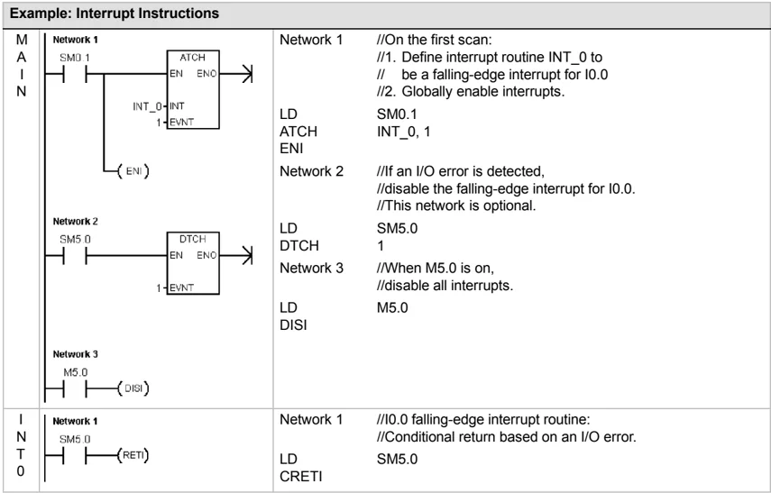
Example: Interrupt Instructions
| MAIN | Network 1SM0.1ATCHEN ENOINT_0-INT1-EVNT(ENI) | Network 1//On the first scan://1. Define interrupt routine INT_0 to// be a falling-edge interrupt for I0.0//2. Globally enable interrupts.LD SM0.1ATCH INT_0, 1ENI |
|---|---|---|
| Network 2SM5.0DTCHEN ENO1-EVNT | Network 2//If an I/O error is detected,//disable the falling-edge interrupt for I0.0.//This network is optional.LD SM5.0DTCH 1 | |
| Network 3M5.0(DISI) | Network 3//When M5.0 is on,//disable all interrupts.LD M5.0DISI | |
| INT 0 | Network 1SM5.0(RET) | Network 1//I0.0 falling-edge interrupt routine://Conditional return based on an I/O error.LD SM5.0CRETI |
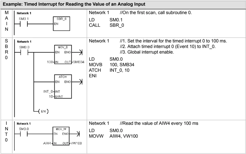
Example: Timed Interrupt for Reading the Value of an Analog Input
| MAIN | Network 1SM0.1SBR_0EN | Network 1//On the first scan, call subroutine 0.LD SM0.1CALL SBR_0 |
|---|---|---|
| SBR 0 | Network 1SM0.0MOV_BEN ENO100-IN OUT-SMB34ATCHEN ENOINT_0-INT10-EVNT(ENI) | Network 1//1. Set the interval for the timed interrupt 0 to 100 ms.//2. Attach timed interrupt 0 (Event 10) to INT_0.//3. Global interrupt enable.LD SM0.0MOVB 100, SMB34ATCH INT_0, 10ENI |
| INT 0 | Network 1SM0.0MOV_WEN ENOAIW4-IN OUT-VW100 | Network 1//Read the value of AIW4 every 100 msLD SM0.0MOVW AIW4, VW100 |
159
S7-200 Programmable Controller System Manual
Example: Clear Interrupt Event Instruction
Network 1 //Instruction Wizard HSC
LD SM0.0 MOVB 16#A0, SMB47 //Set control bits: //write preset;
MOVD +6, SMD52 //PV = 6;
ATCH HSC1_STEP1, 13 //Interrupt HSC1_STEP1: CV = PV for HC1
Network 2 //Clear unwanted interrupts caused //by machine vibration
LD SM0.0 CEVNT 13
160